يشير توزيع إضاءة تركيبات LED إلى توزيع واتجاه وكثافة الضوء المنبعث منها. ويؤثر ذلك بشكل كبير على كفاءة الإضاءة، وكفاءة الطاقة، وراحة البصر. يوفر التوزيع المناسب للضوء إضاءةً وتجانسًا مناسبين، ويوفر الطاقة، ويقلل الوهج، ويعزز السلامة، ويحد من التلوث الضوئي، ويخلق بيئة إضاءة مريحة. ينبغي على شركات إضاءة LED تصميم توزيعات إضاءة مناسبة لضمان مزايا تركيباتها، بينما ينبغي على مهندسي ومصممي الإضاءة اختيار أنماط توزيع إضاءة مناسبة بناءً على الاحتياجات المحددة لتحقيق تأثيرات إضاءة مثالية من تركيبات LED.
عندما يُصدر مصدر ضوء ضوءًا، قد لا يتوافق اتجاه انتشاره مع الاتجاه المتوقع. في هذه الحالات، يلزم تصميم هياكل محددة (مثل العدسات والعاكسات) لتغيير اتجاه انتشار الضوء. يتضمن ذلك ضبط التوزيع المكاني للضوء لتحقيق التأثير المطلوب. تُسمى هذه الطريقة للتحكم في اتجاه انتشار الضوء "منحنى قياس الضوء الضوئي" أو "توزيع الضوء".
يُوضح منحنى توزيع شدة الضوء، المعروف عادةً باسم المنحنى الفوتومتري أو منحنى توزيع الضوء (LDC)، التوزيع المكاني لشدة الإضاءة الصادرة عن التركيبات. يُحصل على منحنى توزيع الشدة مباشرةً من خلال قياسات التركيبات باستخدام مقياس ضوئي. تشمل الصيغ الشائعة لمنحنيات توزيع الشدة IES (في أمريكا الشمالية) وLDT (في أوروبا). بصفتنا مشترين، يُمكننا أيضًا الحصول على هذه الملفات بالتواصل مع مُصنّعي التركيبات. هناك طريقتان لتمثيل المنحنيات الفوتومترية: يُستخدم نظام الإحداثيات المستطيلة عادةً في كشافات الإضاءة، بينما تُستخدم الإحداثيات القطبية للإضاءة الداخلية وإضاءة الطرق.
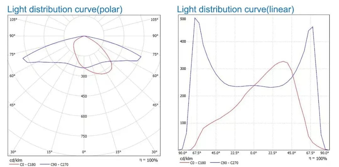
منحنى توزيع الضوء (الإحداثيات القطبية)
في مستوى قياس يمر بمركز مصدر الضوء، تُقاس قيم شدة الإضاءة للتركيبة عند زوايا مختلفة. بدءًا من اتجاه معين، تُحدد شدة الإضاءة عند كل زاوية وتُمثل بمتجهات. يُشكل وصل نهايات هذه المتجهات منحنى توزيع الضوء القطبي/المنحنى الضوئي للتركيبة، كما هو موضح في الجانب الأيسر من الصورة التالية.
منحنى توزيع الضوء (الإحداثيات الخطية)
يُستخدم منحنى التوزيع هذا عادةً لأجهزة مثل مصابيح LED الكاشفة والكشافات. ونظرًا لتركيز أشعة هذه التركيبات بزاوية مصمتة صغيرة جدًا، يصعب تمثيل توزيع شدة الإضاءة المكانية باستخدام الإحداثيات القطبية. لذلك، يستخدم بعض المصنّعين منحنيات توزيع الضوء الإحداثية الخطية/المنحنيات الضوئية لتمثيل توزيع الإضاءة لديهم. يُمثل المحور الرأسي شدة الإضاءة (I)، بينما يُمثل المحور الأفقي زاوية الشعاع، كما هو موضح في الجانب الأيمن من الصورة التالية.
تصنيف نوع توزيع الإضاءة IESNA
منذ تأسيسها عام ١٩٠٦، تتمتع جمعية هندسة الإضاءة في أمريكا الشمالية (IESNA) بتاريخ يمتد لأكثر من قرن. ولا يزال تصنيف توزيعات الإضاءة الذي قدمته IESNA مستخدمًا على نطاق واسع حتى اليوم. نظام تصنيف توزيع التركيبات مُعرّف بوضوح في معيار ANSI/IESNA RP-8-1983. أنواع التركيبات التي تُعرّفها جمعية هندسة الإضاءة في أمريكا الشمالية هي فئات موحدة تُستخدم لوصف أنماط توزيع الإضاءة. تساعد أنواع توزيع الإضاءة هذه متخصصي الإضاءة ومصمميها على فهم كيفية إنتاج التركيبات للضوء وكيفية انتشاره داخل منطقة معينة. تُعرّف IES عدة أنواع توزيع قياسية، يُمثل كل منها رمز من حرفين. تشمل أنواع توزيع تركيبات IES الشائعة النوع الأول، والنوع الثاني، والنوع الثالث، والنوع الرابع، والنوع الخامس، متبوعة بأرقام رومانية (IV)، حيث تُمثل S وM وL القصير، والمتوسط، والطويل على التوالي. يُحدد التصنيف المحدد من خلال 50% ونقاط الكثافة القصوى في ملف IES، والتي سيتم تفصيلها في الأقسام اللاحقة.
يوجد حاليًا العديد من التنسيقات المعيارية للملفات الضوئية، ومن أشهرها EULUMDAT وCIE102 وIESNA LM-63. يُستخدم IESNA LM-63 في أمريكا الشمالية، بينما يُستخدم EULUMDAT في أوروبا، بينما يُستخدم CIE102 في نيوزيلندا. وقد اعتمد المعهد الوطني الأمريكي للمعايير (ANSI) المعيار الحالي لعام 2002 واعترف به. وأصبح IESNA LM-63-2002 تنسيق الملفات الضوئية المخصص لأمريكا الشمالية، بامتداد الملف "*.ies".
تُعرّف أنواع توزيع الإضاءة وفقًا لمعايير IESNA توزيع ضوء التركيبات بدقة أكبر استنادًا إلى شكل المنطقة المُضاءة. بالنسبة لتوزيع الضوء الجانبي، يصف هذا النمط كيفية تشتت الضوء من التركيبة ويتميز بالنقطة التي تصل فيها الكثافة إلى 50%. يتضمن نمط التوزيع هذا قدرة التركيبة على إسقاط الضوء للأمام والخلف. وبعبارات بسيطة، إذا كنت ترغب في إضاءة مسار واحد، فقد يكون النوع الأول مناسبًا؛ وإذا كنت ترغب في إضاءة مسارين، فقد يكون النوع الثاني أكثر ملاءمة. ومع ذلك، فهذه ليست قاعدة صارمة وتتأثر بعوامل مثل ارتفاع التركيب وزاوية الميل وطول الذراع ومسافة التركيبة من حافة الطريق. وقد حددت IESNA خمسة أنماط رئيسية لتوزيع الضوء: النوع الأول والنوع الثاني والنوع الثالث والنوع الرابع والنوع الخامس. تُستخدم هذه التصنيفات عادةً لتحديد الأطياف المناسبة للطرق ذات العرض المتفاوت.
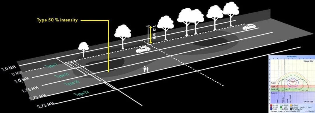
في المعايير الصادرة عن IESNA، يُقسّم الطريق طوليًا إلى خمس مناطق، كما هو موضح في الصورة أعلاه. يُصنّف توزيع الإضاءة الجانبية بناءً على المنطقة التي تقع فيها نقطة شدة الإضاءة القصوى 50%. بالنسبة لمنحنيات توزيع الإضاءة للتركيبات المذكورة أعلاه، إذا كانت نقطة شدة الإضاءة 50% تقع ضمن منطقة النوع الثالث، فإن نوع توزيع الإضاءة المقابل لها يُصنّف ضمن النوع الثالث. من الرسم التخطيطي، يمكننا عمومًا استنتاج أن هذا التوزيع مناسب للطرق ذات المسارات الثلاثة. تُعد توزيعات الإضاءة الجانبية المختلفة مناسبة لمختلف سيناريوهات الاستخدام، كما هو موضح أدناه:
- النوع الأول: ١-١ ميجا هيرتز، عندما يقع مسار شدة ضوء ٥٠١TP3T بين ١ ميجا هيرتز على جانب التركيب وجانب الشارع، يُشار إليه بتوزيع الضوء الضيق المتماثل أو غير المتماثل من النوع الأول. مناسب للأرصفة والممرات والطرق ذات المسار الواحد.
- النوع الثاني: ١-١.٧٥ ميجا هاش، عندما يقع مسار شدة ضوء ٥٠١TP3T بين ١ ميجا هاش و١.٧٥ ميجا هاش على جانب الشارع، يُشار إليه بتوزيع الضوء الضيق غير المتماثل من النوع الثاني. مناسب للطرق ذات المسار الواحد أو المسارين، والطرق الرئيسية، والطرق السريعة.
- النوع الثالث: ١.٧٥-٢.٧٥ ميجا هاش. عندما يقع مسار شدة ضوء ٥٠١TP3T بين ١.٧٥ ميجا هاش و٢.٧٥ ميجا هاش على جانب الشارع، يُطلق عليه اسم توزيع الضوء غير المتماثل الواسع من النوع الثالث. مناسب للطرق الرئيسية والطرق السريعة ومواقف السيارات.
- النوع الرابع: ٢.٧٥-٣.٧٥ ميجا هاش. عندما يقع مسار شدة ضوء ٥٠١TP3T بين ٢.٧٥ و٣.٧٥ ميجا هاش على جانب الشارع، يُطلق عليه اسم توزيع الإضاءة الأمامية غير المتماثلة من النوع الرابع. مناسب لمواقف السيارات، والساحات، وإضاءة المناطق المثبتة على الجدران.
- النوع الخامس: نمط دائري متناسق، مع توزيع دائري متناسق حول التركيبة، مما يوفر توزيعًا متساويًا للضوء في الأمام والخلف. مناسب لإضاءة مواقف السيارات والمناطق المحيطة.
توزيع الضوء الرأسي والطولي
يشير توزيع الضوء الرأسي إلى توزيع الضوء الرأسي للتركيبة، بناءً على موضع أقصى شدة ضوئية (مقاسة بالشمعة) في الشبكة الموازية لـ TRL. ينقسم الطريق على طول TRL إلى مناطق مختلفة وفقًا لمسافته من TRL (معبرًا عنها كمضاعفات لارتفاع التركيب). يتضمن توزيع الضوء الطولي قدرة التركيب على إسقاط الضوء على الجانبين الأيسر والأيمن، والذي يتم تحديده من خلال نقطة أقصى شدة للتركيب. وفقًا لتعريف IESNA، تنطبق فئة "S" على مسافات الأعمدة التي تقل عن 2.25 مرة من ارتفاع التركيب، وتنطبق "M" على مسافات الأعمدة بين 2.25 و3.75 مرة، وتنطبق "L" على مسافات الأعمدة بين 3.75 و6.0 مرات. ومع ذلك، فهذه ليست قاعدة صارمة وتتأثر بعوامل مثل ترتيب التركيب وظروف الطريق. بشكل عام، تكون التركيبات المصنفة على أنها "S" مناسبة لمسافات أعمدة أصغر، بينما تكون التركيبات المصنفة على أنها "L" مناسبة للمسافات الأكبر.
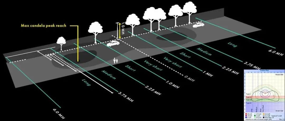
في المعايير الصادرة عن IESNA، يُقسّم الطريق عرضيًا إلى ثلاث مناطق، كما هو موضح في الصورة أعلاه. يُصنّف توزيع الإضاءة الطولي بناءً على المنطقة التي تقع فيها نقطة أقصى شدة إضاءة 100%. بالنسبة لمنحنيات توزيع الإضاءة للتركيبات الموضحة، إذا كانت نقطة أقصى شدة إضاءة لإضاءة الشارع تقع ضمن منطقة "المتوسطة"، يُصنّف نوع توزيع الإضاءة المقابل لها على أنه "متوسط من النوع الثاني". من الرسم التخطيطي، يمكننا استنتاج أن نمط توزيع الإضاءة هذا يتميز بمسافة بين الأعمدة تبلغ حوالي 3.0-3.5 أضعاف ارتفاع العمود. تختلف توزيعات الإضاءة الطولية باختلاف سيناريوهات تباعد الأعمدة، كما هو موضح أدناه:
- مقابل، 0-1.0 MH: عندما يقع مسار شدة الضوء 100% بين 0 إلى 1.0 MH في خطوط الطريق العرضية، يشار إلى ذلك باسم توزيع الضوء الطولي VS (قصير جدًا).
- س، 1.0-2.25 MH: عندما يقع مسار شدة الضوء 100% بين 1.0 إلى 2.25 MH في خطوط الطريق العرضية، يشار إليه باسم توزيع الضوء الطولي S (القصير).
- م، 2.25-3.75 MH: عندما يقع مسار شدة الضوء 100% بين 2.25 إلى 3.75 MH في خطوط الطريق العرضية، يشار إليه باسم توزيع الضوء الطولي M (متوسط).
- ل، 3.75-6.0 MH: عندما يقع مسار شدة الضوء 100% بين 3.75 إلى 6.0 MH في خطوط الطريق العرضية، يشار إليه باسم توزيع الضوء الطولي (L).
- في إل، >6.0 MH: عندما يقع مسار شدة الضوء 100% خلف 6.0 MH في خطوط الطريق العرضية، يشار إلى ذلك بتوزيع الضوء الطولي VL (طويل جدًا).
خصائص تطبيق توزيع الضوء الطولي
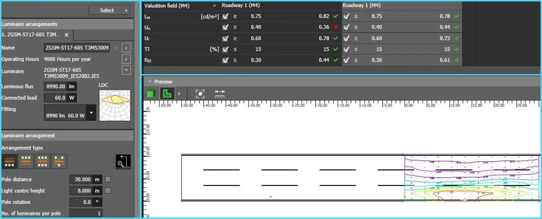
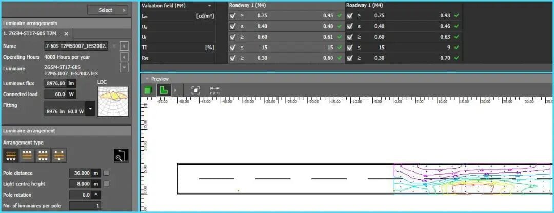
لقد استخدمنا DIALux evo لتحليل تطبيقات مصابيح الشوارع من النوع II S والنوع II M.
حالة الطريق هي كما يلي: عرض 7 أمتار، ثلاثة مسارات، بروز 0.8 متر، ارتفاع العمود 8 أمتار، تباعد التركيبات 36 مترًا، وفقًا لمستوى الإضاءة EN13201 M4.
بعد استيراد البيانات الضوئية للنوع II S والنوع II M إلى DIALux evo للتحليل، كانت النتائج واضحة للغاية. بالنسبة للبيانات الضوئية للنوع II S، وجد أن توزيع الضوء الطولي قصير نسبيًا ويفشل في توزيع الضوء بشكل فعال على جوانب التركيبات. لذلك، يجب تقليل المسافة بين التركيبين إلى 33 مترًا لضمان حصول الموضع الأوسط بينهما على إضاءة كافية. هذا التعديل ضروري لتلبية التوحيد المطلوب. في المقابل، يعمل توزيع النوع II M بشكل أفضل في هذا الصدد مع تباعد التركيبات البالغ 36 مترًا، وتفي جميع معلمات المحاكاة بمعايير M4. يبلغ التباعد البالغ 36 مترًا 4.5 أضعاف ارتفاع التركيب، وهو ما يتجاوز قليلاً 3.75 مرة الموصى به من قبل IESNA. وبالتالي، يُنصح باستخدام نتائج محاكاة الإضاءة كأساس للاختيار النهائي للتركيبات.
يُقدّم ما سبق بشكلٍ رئيسي مفهوم توزيع الإضاءة وفقًا لمعايير IESNA، مُغطّيًا توزيعات الأنواع الأول والثاني والثالث، بالإضافة إلى مفاهيم أنواع توزيع الإضاءة القصيرة والمتوسطة والطويلة، ويُقدّم بإيجاز تطبيقاتها العملية. يُمكن فهم هذه المفاهيم من تحديد نوع القياس الضوئي المُناسب للمشروع بسرعة. على سبيل المثال، يُناسب توزيع النوع الثاني الطرق ذات المسار الواحد أو المسارين، بينما يُناسب توزيع النوع القصير الحالات التي تكون فيها المسافة بين الأعمدة ثلاثة أضعاف ارتفاع التركيب. أما توزيع النوع المتوسط، فيُناسب المسافات بين الأعمدة أربعة إلى خمسة أضعاف ارتفاع التركيب. وبالطبع، هذه ليست معايير مطلقة، ويجب التحقق منها باستخدام برنامج DIALux أو أي برنامج آخر لمحاكاة إضاءة الطرق.